Basic Neural Net from "Scratch"
This notebook can be found in this kaggle notebook.
You can use this article as a reference to the kaggle notebook but the same notes will appear in kaggle.
Overview
This notebook is an example of building a Neural Network from “scratch”.
Specifically, it goes through Chapter 4 of the excellent book Deep Learning for Coders with fastai & PyTorch.
Notes or descriptions above or below cells may differ from the book to fit my own narrative of understanding.
!pip install fastbook
!pip install fastai
fastai and fastbook are libraries created by the authors of Deep Learning for Coders with fastai & PyTorch.
These libraries are not only appropriate for the book, but are designed to be used in personal and production level projects.
As another aside, yes import * is usually bad practice, but for notebooks, this tends to be the norm.
from fastai.vision.all import *
from fastbook import *
Learning Objectives
The objective in this notebook is demontrate the process of building a Neural Network from “scratch”.
In practice, this means identifying the process of training a Neural Network as well as implementing the basic coding requirements.
The diagram below shows the training process of a Neural Network. This will act as our guide for building our Neural Network.
#id gradient_descent
#caption The gradient descent process
#alt Graph showing the steps for Gradient Descent
gv('''
init->predict->loss->gradient->step->stop
step->predict[label=repeat]
''')

The next sections will implement the above diagram. This diagram is the basis of all neural networks. There will be a summary at the end with this diagram, detailing the actions taken with the steps in the diagram.
Download MNIST
For our Neural Network, we are going to train an Image Recognition Model.
We are going to use the MNIST data set, which is a dataset that contains images of handwritten numbers.
Our model is going to identify whether an image is a 3 or a 7.
path = untar_data(URLs.MNIST_SAMPLE)
(path/'train').ls()
(#2) [Path('/root/.fastai/data/mnist_sample/train/7'),Path('/root/.fastai/data/mnist_sample/train/3')]
(path).ls()
(#3) [Path('/root/.fastai/data/mnist_sample/valid'),Path('/root/.fastai/data/mnist_sample/labels.csv'),Path('/root/.fastai/data/mnist_sample/train')]
Setting up the training data
In this section, we are going to focus on setting up our training and validation data.
In the training of our Neural Network, we are obviously going to use our training data to train the model but we are going to use a validation set during the training of the model to test the accuracy/improvements of the model.
The validation set, is a set of inputs and labels that the model hasn’t “seen”, meaning it’s not part of the training data and will be used to calculate our LOSS.
What’s happening?
We are going to need to make sure all images have the same size. This is essential for training the model correctly.
We are going to set all images to a pixel size of 28 * 28 which is 255.
PIXEL_SIZE = 28*28
What’s happening?
We are going to open each image and save each image into a rank2 tensor.
Each list in the rank2 tensor will represent a x-axis and y-axis. These axes represent pixels in the image.
We are creating x2 rank2 tensors - training and validation.
training_data = (path/'train').ls().sorted()
validation_data = (path/'valid').ls().sorted()

# Open each image and insert into a rank2 tensor
def extract_images(image_folder_path):
    return {path.name: [tensor(Image.open(x)) for x in path.ls()] for path in image_folder_path}

training_images = extract_images(training_data)
validation_images = extract_images(validation_data)
type(validation_images)
dict
Explanations
What is a tensor?
A tensor is a multi-dimensional array.
Under the hood, in our context, it’s usually a Numpy ndarray. Basically, a multi-dimensional array that makes it easy to perform matrix multiplication and addition with access to a GPU.
What is a rank2 tensor?
A rank2 tensor, is a tensor that represents a matrix.
The matrix can be represented as a list of lists. Usually just a x-axis list and a y-axis list.
[[x axis], [y axis]]
What’s happening?
Using access to the .shape variable, we can view the “shape” of the tensor.
This indicates a tensor of a x and y axis of 28 respectively, matching our Pixel Size of 28*28
torch.Size([28, 28])
We also have a helper function show_image, will print out one of our images.
validation_images['7'][0].shape
torch.Size([28, 28])
show_image(validation_images['7'][-1])
<Axes: >

What’s happening?
How we use our training data is a key question.
The goal is to train a Neural Network to classify an unseen image, a 3 or a 7. In this case, how will the model know what a 3 or 7 looks like?
The following approach “stacks” all the images of a 3 and “stacks” all the images of a 7.
This creates an “ideal” image. This can also be thought of as an average of a 3 or a 7. By creating this “ideal”, the Neural Network can learn to compare the pixel values of an input against the “ideal” image of a 3 or 7, thus determining a probability of either number.
We stack the images to create the ideal/optimal version of the 3 and 7. We’ll divide the tensor by 255 to represent RGB. By stacking the tensors, we are creating a rank3 tensor. A tensor of matrices.
def stack_tensors(image_tensors):
    return {t: torch.stack(image_tensors[t]).float()/255 for t in image_tensors.keys()}
stacked_tensors = stack_tensors(training_images)
show_image(stacked_tensors['7'].mean(0))
<Axes: >

stacked_tensors['7'].ndim
3
Explanations
What is a rank3 tensor?
A rank3 tensor is a list of matrices,aka a tensor of rank2 tensors e.g.
[
[[a, b], [c,d]],
[[e, f], [g, h]],
]
What’s happening?
We are combining and concatenating x2 rank3 tensors into one rank2 tensor.
Cat doesn’t create a new dimension but we are telling Pytorch to infer the size of the dimensions using -1.
The rank3 tensors are essentially a list of rank2 tensors. We are combining all the training data into a new tensor for both 3 and 7. All the training data are rank2 tensors, so combined, they just make a new big rank2 tensor.
When we print the shape we see, [12396, 784]. This means we are seeing 12396 items (images) of a size 784 each, which is the pixel size 28 * 28.
This be will be the x-axis for our training data.
train_x = torch.cat([stacked_tensors['3'], stacked_tensors['7']]).view(-1, PIXEL_SIZE)
train_x.shape
torch.Size([12396, 784])
train_x.ndim
2
What’s happening?
We are creating a rank2 tensor which will be our y axis.
This represents whether a cell is a 3 or 7.
1 will be the label for the image 3 and a 0 will be the label for the image 7.
When we print the shape we see [12396, 1]. This means we have 12396 labels (representing each image) that have the label value 1 or a 0, in other words a 3 or a 7.
We then combine our training sets into an x and y axis.
train_y = tensor([1]*len(stacked_tensors['3']) + [0]*len(stacked_tensors['7'])).unsqueeze(1)
train_y.shape
torch.Size([12396, 1])
dset = list(zip(train_x,train_y))
x,y = dset[0]
We repeat the same process for our validation set.
stacked_valid_tensors = stack_tensors(validation_images)
valid_x = torch.cat([stacked_valid_tensors['3'], stacked_valid_tensors['7']]).view(-1, PIXEL_SIZE)
valid_x.shape
torch.Size([2038, 784])
We create a validation DataLoader object with a batch size of 256.
The DataLoader class is a fastAI class that is a helpful wrapper around loading and batching training/validation data.
valid_y = tensor([1]*len(stacked_valid_tensors['3']) + [0]*len(stacked_valid_tensors['7'])).unsqueeze(1)
valid_dset = list(zip(valid_x,valid_y))
valid_dl = DataLoader(valid_dset, batch_size=256)
Understanding the loss function
This simple example shows how we can create predictions using a linear function: y = mx + b and a loss function to measure the accuracy of our predictions.
The PARAMETERS of the linear function are m and b - weights and bias. We can first generate random values for variables since we will adjust them according to the calculated gradients.
def init_params(size, std=1.0):
    return (torch.randn(size)*std).requires_grad_()

weights = init_params((PIXEL_SIZE,1))
bias = init_params(1)
weights.mean(), bias.mean()
(tensor(0.0235, grad_fn=<MeanBackward0>),
tensor(0.3472, grad_fn=<MeanBackward0>))
Basic Loss Function Explained
This is an example of the loss function calculation. The generated predictions that are closer to 0, mean the input is a 7 and the predictions closer to 1 mean its a 3.
In the example, the targets are [1, 0 ,1] == [3, 7, 3] and the predictions are [0.9, 0.4, 0.2] == [3, 7, 7].
The last prediction is incorrect.
trgts = tensor([1,0,1])
prds = tensor([0.9, 0.4, 0.2])
torch.where(trgts==1, 1-prds, prds) will use C/CUDA to perform essentially a list comprehension on the matrix. But the logic goes as follows:
If the value at an index in
trgts[i]results in the value being equal to1e.g.trgts==1is true, then the value is a3, then return the first argument path (1-prds)1-prdsreturns the difference between the target and the prediction by subtracting 1 (meaning the iamge of a 3) from the prediction. This is the accuracy for the prediction of a 3. So in our first case, the target is 1 (an image of a 3) and the prediction is a 0.9 (so very certain its a 3). By subtracting1 - 0.9, we get0.1. Remember this is a Loss function, so the lower the value the more accurate and in this case, its very accurateIf the value at an index in
trgts[i]doesn’t equal 1, meaning its 0 (meaning the image is a 7), then return the second argument path without modifyingprds, this will essentially be the distance from 0 (the distance from an image of a 7). So in this example, the prediction for the 7 in the middle index was0.4, so the distance from0is0.4, therefore the prediction is fairly accurateThe last item in
trgtsis a 1 (meaning its an image of a 3), the prediction is a0.2(meaning its closer to a 7). Since the target is 1, it returns1-prds, the difference is0.8. Remember this is a Loss function, so this is a very inaccurate prediction
torch.where(trgts==1, 1-prds, prds)
tensor([0.1000, 0.4000, 0.8000])
We can see the mean accuracy for our loss function is 0.4333
torch.where(trgts==1, 1-prds, prds).mean()
tensor(0.4333)
If we change the last prediction to be more accurate (from 0.2 to 0.8), we can see the loss decrease since this is now more accurate.
trgts = tensor([1,0,1])
prds = tensor([0.9, 0.4, 0.8])
torch.where(trgts==1, 1-prds, prds)
tensor([0.1000, 0.4000, 0.2000])
torch.where(trgts==1, 1-prds, prds).mean()
tensor(0.2333)
The problem here, is that our loss function assumes all values of the predictions will always be between 0 and 1.
Let’s change the value of the last index of predictions to 3.
trgts = tensor([1,0,1])
prds = tensor([0.9, 0.4, 3])
We can see here the prediction for the last index is -2.000 which becomes meaningless and a mean loss accuracy of -0.5000.
torch.where(trgts==1, 1-prds, prds)
tensor([ 0.1000, 0.4000, -2.0000])
torch.where(trgts==1, 1-prds, prds).mean()
tensor(-0.5000)
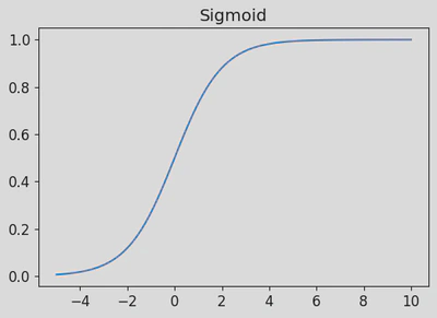
Sigmoid Function
To ensure that the values of the loss function are usable and fit between 0 and 1.
We can use a sigmoid function to map our prediction values to fit 0 to 1.
The sigmoid formula:
eis eulers number which is the natural logarithm of a value2.71828
plot_function(torch.sigmoid, title='Sigmoid', min=-5, max=10)
In the prds tensor, we add values below 0 and above 1.
trgts = tensor([1,0,1])
prds = tensor([-0.9, 0.4, 3])
prds
tensor([-0.9000, 0.4000, 3.0000])
We can observe, that by applying the sigmoid function to the prds tensor, it will convert all the values that are outside of the range 0-1 to 0-1.
Importantly, the higher the predictions, the higher the value is closer to 1 and inversly when negative values.
prds.sigmoid()
tensor([0.2891, 0.5987, 0.9526])
Creating the loss function
Now we can create our loss function. We know we need to apply the sigmoid function to the predictions to map them between 0-1.
We can calculate the loss as a distance from the our target predictions (0 for 7 and 1 for 3).
Remember, the lower the value of the loss function, the more accurate. The sigmoid function is essentially our activation function.
def mnist_loss(predictions, targets):
    predictions = predictions.sigmoid()
    return torch.where(targets==1, 1-predictions, predictions).mean()
Explanations
What is an Activation Function?
An activation function is a function that introduces non-linearity between the different levels in a Neural Network.
Think of a Neural Network as a continuous linear line on a graph. The Activation Functions, will introduce bends in the line, in order to be able to fit or model a complex data set.
Batching, Training Epochs and Optimization (Stochastic Gradient Descent)
Now we need to be able to iteratively train the model and lower the loss function by training in epochs.
First we’ll need to split our data into batches.
The reason behind using batching is, that if we trainined our whole dataset in one go, it will be slow and time consuming and the GPU may even run out of memory. If we only train on one item, its going to be a very inaccurate model.
On each epoch, we essentialy create a new “sample” of random training data in a new batch.
batch = train_x[:4]
batch.shape
torch.Size([4, 784])
Prediction Function
We are going to create our prediction function y = mx + b.
An important note below. @ allows Pytorch to perform matrix multiplication, and uses C/CUDA
def linear_func(input_batch):
    """
    Compute the linear transformation of the input batch.

    Args:
        input_batch (tensor): Input batch of data, where each row represents a single data point.

    Returns:
        tensor: The result of the linear transformation applied to the input batch,
                with the bias vector added.
    """
    return input_batch@weights + bias
We will initialize our randomized weights and bias.
def init_params(size, std=1.0):
    return (torch.randn(size)*std).requires_grad_()

weights = init_params((PIXEL_SIZE,1))
bias = init_params(1)

weights.mean(), bias.mean()
(tensor(-0.0128, grad_fn=<MeanBackward0>),
tensor(-0.2762, grad_fn=<MeanBackward0>))
preds = linear_func(batch)
preds
tensor([[23.6921],
[ 2.4338],
[19.6201],
[ 3.7629]], grad_fn=<AddBackward0>)
Lets calculate the loss on the predictions:
labels_batch = train_y[:4]
loss = mnist_loss(preds, labels_batch)
loss, labels_batch
(tensor(0.0258, grad_fn=<MeanBackward0>),
tensor([[1],
[1],
[1],
[1]]))
We can see our loss, lets call backward() (backpropogation) to calculate the derivatives/gradients so we can determine how much we need to change our parameters.
loss.backward()
weights.grad.shape, weights.grad.mean(), bias.grad
(torch.Size([784, 1]), tensor(-0.0024), tensor([-0.0241]))
Lets encapsulate calculate gradients into a function:
def calc_grads(xb, yb, model):
    preds = model(xb)
    loss = mnist_loss(preds, yb)
    loss.backward()
calc_grads(batch, labels_batch, linear_func)
weights.grad.mean(), bias.grad
(tensor(-0.0049), tensor([-0.0482]))
We need to be able to reset our calculated gradients on each iteration otherwise, they gradients will just be added to each other. We’ll use the zero function on the tensors:
weights.grad.zero_()
bias.grad.zero_()
tensor([0.])
Lets load our training data into a DataLoader for easier access.
training_dl = DataLoader(dset, batch_size=256)
Lets create a training epoch function.
For the training data, its going to go through each x and y in the batch (x is the data and y is the correct label) and calculate the gradients/derivatives based on the loss function of the predictions. We then step the weights so that our weights and bias become more accurate.
def train_epoch(dl, lr, model):
    for xb, yb in dl:
        calc_grads(xb, yb, model)
        weights.data -= weights.grad * lr
        bias.data -= bias.grad *lr
        weights.grad.zero_()
        bias.grad.zero_()
We also want some metric to view the accuracy of the predictions. We can just check if a value is greater than 0 (meaning its a 3) and if its a 0 its a 7. This will compare it the label in train_y (either a 0 or 1)
(preds>0.0).float() == train_y[:4]
tensor([[True],
[True],
[True],
[True]])
We can create a batch accuracy function to tell us the accuracy of the predictions:
def batch_accuracy(xb, yb):
    """
    Calculate the accuracy of predictions for a batch of data.

    Args:
        xb (Tensor): Predicted probabilities for each sample in the batch.
        yb (Tensor): Ground truth labels for each sample in the batch.

    Returns:
        Tensor: Mean accuracy of predictions for the batch.

    Explanation:
        This batch accuracy function measures the accuracy of the predictoins.
        If the prediction is less than 0.5 its closer to a 0 (meaning a 7).
        (preds>0.5) resolves to a bool and yb is the y axis for the truth label.
        e.g.
        If prediction is < 0.5 its False (meaning a 7) and if yb is a 0 (meaning a 7), then this prediction is correct.
        If prediction is > 0.5 its True (meaning a 3) and if yb is a 1 (meaing a 3), then this prediction is correct
    """
    preds = xb.sigmoid()
    correct = (preds>0.5) == yb
    return correct.float().mean()
batch_accuracy(linear_func(batch), train_y[:4])
tensor(1.)
We can create a validate epoch function that will make predictions on the validation set and measure the accuracy of those predictions. It’s important to use the validation set and NOT the training set. This is essentially “unseen” data by the model, so it’s a very accurate way to determine if the model is accurate.
def validate_epoch(model):
    accs = [batch_accuracy(model(x), y) for x,y in valid_dl]
    return round(torch.stack(accs).mean().item(), 4)
validate_epoch(linear_func)
0.5748
Now we can train the model based on a number of epochs and after each epoch we can measure the accuracy of the predictions using the validation set using validate_epoch
lr = 0.1
for i in range(20):
    train_epoch(training_dl, lr, linear_func)
    print(validate_epoch(linear_func), end=' ')
0.7253 0.8163 0.8473 0.8683 0.88 0.8907 0.902 0.9103 0.9162 0.9206 0.9226 0.925 0.929 0.9319 0.9334 0.9344 0.9378 0.9397 0.9417 0.9431
This part covers calculating the loss function on the predictions, calculating the gradients of the loss function towards the targets and stepping the weights and bias according to the gradients and learning rate to fine tune the input to make more accurate predictions.
Creating an optimizer
We are going to use some Pytorch and FastAI functions/objects to make things easier.
The below optimizer simply contains our model weights and learning rate. It will encapsulate the step to update params according to the gradients and also to zero out the gradients.
class BasicOptim:
    def __init__(self, params, lr):
        self.params, self.lr = list(params), lr

    def step(self, *args, **kwargs):
        for p in self.params:
            p.data -= p.grad.data * self.lr

    def zero_grad(self, *args, **kwargs):
        for p in self.params:
            p.grad = None
nn.Linear (neural net.Linear) contains the linear function we have been using as well as the parameters. It does the same thing as our init_params function. It will randomly initilize weights and bias
linear_model = nn.Linear(PIXEL_SIZE, 1)
w,b = linear_model.parameters()
w.shape,b.shape
(torch.Size([1, 784]), torch.Size([1]))
We can make a basic Optimizer. The optimizer contains our steps to update our model params and the learning rate.
opt = BasicOptim(linear_model.parameters(), lr)
We can redefine train_epoch to use the the optimizer.
def train_epoch(model, opt):
    for xb, yb in training_dl:
        calc_grads(xb, yb, model)
        opt.step()
        opt.zero_grad()
validate_epoch(linear_model)
0.215
def train_model(model, opt, epochs):
    for i in range(epochs):
        train_epoch(model, opt)
        print(validate_epoch(model), end=' ')
train_model(linear_model, opt, 20)
0.5352 0.8623 0.936 0.9536 0.9633 0.9633 0.9652 0.9667 0.9682 0.9687 0.9687 0.9696 0.9701 0.9711 0.9716 0.9716 0.9716 0.9726 0.9726 0.9726
Now we can use the fastai Learner object which encapsulates everything we’ve built. The DataLoaders class will contain both our training and validation sets. We’ll also redefine the linear model so we can start with fresh randomized params. We’ll also use SGD (Stochastic Gradient Descent) optimizer from fastai, since we’ve been basically implementing this from scratch this whole time.
linear_model = nn.Linear(PIXEL_SIZE, 1)
dls = DataLoaders(training_dl, valid_dl)
learn = Learner(dls, linear_model, opt_func=SGD,
                loss_func=mnist_loss, metrics=batch_accuracy)
Explanations
Learner is a fastAI class that encapsulates everything required to train a Neural Network:
dls: Dataloaders for the training and validation setsmodel: The model used for predictionsopt_func: The optimization function/method, in our case, Stochastic Gradient Descentloss_func: Our function to calculate the lossmetrics: Our human readable function to present the accuracy of our model to the reader
To run the equivalent of train_model, we call learn.fit with the epoch and learning rate.
lr = 0.1
learn.fit(10, lr=lr)
| epoch | train_loss | valid_loss | batch_accuracy | time |
|---|---|---|---|---|
| 0 | 0.216353 | 0.373136 | 0.535329 | 00:00 |
| 1 | 0.120997 | 0.182699 | 0.873405 | 00:00 |
| 2 | 0.083601 | 0.106391 | 0.937684 | 00:00 |
| 3 | 0.065680 | 0.079394 | 0.955839 | 00:00 |
| 4 | 0.055948 | 0.066364 | 0.963690 | 00:00 |
| 5 | 0.050042 | 0.058729 | 0.965162 | 00:00 |
| 6 | 0.046086 | 0.053686 | 0.966634 | 00:00 |
| 7 | 0.043211 | 0.050082 | 0.966634 | 00:00 |
| 8 | 0.040988 | 0.047358 | 0.969087 | 00:00 |
| 9 | 0.039190 | 0.045215 | 0.969087 | 00:00 |
#id gradient_descent
#caption The gradient descent process
#alt Graph showing the steps for Gradient Descent
gv('''
init->predict->loss->gradient->step->stop
step->predict[label=repeat]
''')

To summarize the whole fundementals of Deep Learning:
- Initialize random parameters (weights and bias) for the Neural Network model
- Create predictions using a model (linear function) and weights and bias
- A Neural Network is made up of linear functions and ReLU (rectified linear units) or activation functions
- Calculate the loss on the predicions, this gives us a measurement of the performance of the predictions
- Calculate the gradients/derivatives of the loss, this gives us the required magnitude and direction to move the weight and biases towards the correct prediction
- Step the weights, reduce the weights and bias by the gradients * the learning rate, this should make the weights and bias more accurate in predictions
- Repeat for x number of epochs
Building our own Learner
This section is an optional section where I’m just playing around with creating a custom Learner class.
Things we need:
- dls
- neural net
- optimizer
- loss function
- metrics
functions we need:
- fit
class CustomLearner:
    def __init__(self, training, validation, neural_net, optimizer, loss, metrics):
        self.training = training
        self.validation = validation

        self.neural_net = neural_net
        self.optimizer = optimizer

        # TODO: 4. TRy a different loss function
        self.loss = loss

        # TODO: 5. Try a different metric function?
        self.metrics = metrics

    def fit(self, epochs):
        for i in range(epochs):
            self._train_epoch()
            # TODO 6. Make this pretty print
            print(self._validate_epoch(), end=' ')

    def _train_epoch(self):
        for xb, yb in self.training:
            self._calc_grads(xb, yb)
            self.optimizer.step()
            self.optimizer.zero_grad()

    def _calc_grads(self, xb, yb):
        preds = self.neural_net(xb)
        loss = self.loss(preds, yb)
        loss.backward()

    def _validate_epoch(self):
        accs = [self.metrics(self.neural_net(x), y) for x,y in self.validation]
        return round(torch.stack(accs).mean().item(), 4)
linear_model = nn.Linear(PIXEL_SIZE, 1)
opt = BasicOptim(linear_model.parameters(), lr)
dls = DataLoaders(training_dl, valid_dl)
learn = CustomLearner(training=dls[0], validation=dls[1], neural_net=linear_model, optimizer=opt, loss=mnist_loss, metrics=batch_accuracy)
learn.fit(10)
0.5479 0.8769 0.9365 0.9565 0.9638 0.9638 0.9662 0.9682 0.9696 0.9691
We can also use the FastAI SGD in our custom learner
linear_model = nn.Linear(PIXEL_SIZE, 1)
sgd = SGD(linear_model.parameters(), lr)
learn = CustomLearner(training=dls[0], validation=dls[1], neural_net=linear_model, optimizer=sgd, loss=mnist_loss, metrics=batch_accuracy)
learn.fit(10)
0.5635 0.8784 0.9374 0.9555 0.9638 0.9638 0.9657 0.9667 0.9682 0.9691
Lets create a custom linear_model, this example creates a neural net of 19 layers? Just seeing what would happen.
simple_net = nn.Sequential(
    nn.Linear(PIXEL_SIZE, 30),
    nn.ReLU(),
    nn.Linear(30, 30),
    nn.ReLU(),
    nn.Linear(30, 30),
    nn.ReLU(),
    nn.Linear(30, 30),
    nn.ReLU(),
    nn.Linear(30, 30),
    nn.ReLU(),
    nn.Linear(30, 30),
    nn.ReLU(),
    nn.Linear(30, 30),
    nn.ReLU(),
    nn.Linear(30, 30),
    nn.ReLU(),
    nn.Linear(30, 30),
    nn.ReLU(),
    nn.Linear(30, 1),
)
sgd = SGD(simple_net.parameters(), lr)
learn = CustomLearner(training=dls[0], validation=dls[1], neural_net=simple_net, optimizer=sgd, loss=mnist_loss, metrics=batch_accuracy)
learn.fit(10)
0.5068 0.5068 0.5068 0.5068 0.5068 0.5068 0.5068 0.5068 0.5068 0.5068
From our results, after 10 epochs, its not very accurate.
If we redefine our neural net just using 3 layers, its much more accurate in 10 epochs.
simple_net = nn.Sequential(
    nn.Linear(PIXEL_SIZE, 30),
    nn.ReLU(),
    nn.Linear(30, 1)
)
sgd = SGD(simple_net.parameters(), lr)
learn = CustomLearner(training=dls[0], validation=dls[1], neural_net=simple_net, optimizer=sgd, loss=mnist_loss, metrics=batch_accuracy)
learn.fit(10)
0.5068 0.8066 0.9189 0.9438 0.9574 0.9638 0.9657 0.9672 0.9687 0.9701
Using a 3 layer net, is much more accurate in 10 epochs