Language Models

Language Models are Neural Networks that are used to classify text or to predict/generate text depending on the context.

Overview

An LM first requires the following pre-processing.

Tokenization

The purpose of Tokenization is to split a corpus (texts) into tokens.

These tokens will eventually be converted to a numeric form suitable for training in a Neural Network (Numericalization).

The tokens can be split in different ways, such as Word Tokenization, with the most common being Subword Tokenization.

The purpose of Tokenization is to be able to build a vocabulary of the most frequent words/subwords. These tokens will build the vocabulary and will be used to predict or classify a text.

Word Tokenization

Word Tokenization will split a text/corpus by words, usually by a white space.

This is a naive Tokenization strategy since there are different languages that don’t use white spaces in the same way as the English Language.

Furthermore, Word Tokenization maybe less efficient in generalization and generation/prediction since it needs to build a vocabulary of whole words, instead of the most common subwords that could appear in many different words e.g. wording vs ing, a token of ing could be applied to many differnt words.

Subword Tokenization

Subword Tokenization is a Tokenization strategy that builds a vocabulary on the most frequent subwords e.g. ing.

This avoids the issue of splitting by whitespace. This has the greater potential for generalization of words and can be used in different languages.

Special Tokens

Using the FastAI library, the Tokenizer introduces special tokens to the text.

• xx***: Indicates a special token
• xxbos: Indicates the beginning of a text, “beginning of a stream”
• xxmaj : Indicates the following word is capitalized
• xxunk: Unknown word

These special tokens are useful because it helps with the training. xxbos will indicate the start of the stream, so when we split and shuffle the training data, we only split and shuffle according to streams. This way, the context when training on the text is not lost and remains coherent.

Numericalization and Vocabulary

Numericalization is the stage of preprocessing where the Tokens are converted into normalized and compatible numbers for training in a matrix.

The vocabulary is a data structure that is created using the tokens with a numerical value.

The numerical value is what is used in the training process. Those values map to the tokens in the vocabulary.

e.g.

{"ing": 0, "the": 1, "of": 2, ...,}

An example of how a matrix of tokens might map to the numerical values via the Vocabulary:

[['xxunk','xxpad','xxbos','xxeos','xxfld','xxrep','xxwrep','xxup','xxmaj','the',',','.','and','a','of','to','is','in','it','i'...]"

TensorText([   2,    8,    0,    8,    0, 1269,    9, 1270,    0,   14,    8,    0,    8,    0,   12,    8,    0,    8,    0,   15])

RNN

Recurrent Neural Networks are one of the foundational Language Models.

RNNs are characterized as Neural Networks that have “contextual long-term memory”.

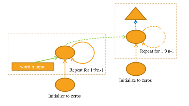
An RNN will have a “hidden state” that is persistent during training, this is the “long-term memory”.

This hidden state will be mutated and persisted in a forward pass on each input.

RNNs unlike basic Neural Networks use a loop in the forward pass to mutate and persist the hidden state when training a batch.

Without the loop and persistent hidden state, a Neural Network would not be able to learn a sequential context as efficiently.

Back Propagation Through Time

Back Propagation Through Time is the required Back Propagation technique for RNNs.

It is pretty much the same procedure as Back Propagation in a basic Neural Network, but we need to use the Hidden State at each stage of Back Propagation, this represents the “time” element.

To apply BPTT, the RNN needs to be “unfolded”. This essentially means creating a deep feed forward network.

Each layer needs to be copied into a computational in-memory graph. Essentially, each iteration in the RNN loop needs to be recreated, using each stages input and hidden state in order to compute the gradients for the weights which are applied to all layers.

This obviously the drawback of creating a large in-memory structure.

Exploding/Vanishing Gradient

RNNs are subject to the Exploding/Vanishing Gradient problem as multiple RNN layers are used.

The deeper the Neural Network, the more likely this issue is to occur.

The Exploding/Vanishing Gradient problem is when Gradients are propagated back through the Neural Network and they eventually “explode” towards a extremely large number or are diminished to an extremely small number towards 0.

Either way, this extremely small Gradient or extremely large Gradient has negative effects in training.

A large Gradient will effectively overshoot an adjustment for the weights and bias and a small Gradient will not update the weights/bias in a significant manner.

Since Neural Networks are essentially networks that perform matrix multiplication, a deep network will perform matrix multiplication at each layer, causing an acceleration or deceleration depending on the scalar.

Long Short-Term Memory

A LSTM RNN is used to mitigate the Exploding/Vanishing Gradient problem.

LSTM introduces a new state alongside side the hidden state - the “cell state”.

The cell state is a persistent state that is NOT used in the matrix multiplication, but instead uses addition alongside the products of the input and hidden state.

This ensures, the cell state is not subject to the Exploding/Vanishing Gradient problem since the cell state only uses addition.

LSTM uses x2 activation functions:

• Sigmoid: Converts input between {0, 1}
• Tanh: Converts input between {-1, 1}

LSTM uses x4 gates which are used for specific purposes:

• Forget Gate: Decides which information to drop from the long term memory (cell state)

• Input Gate: Decides which new information to store in the cell state

• Cell Gate: Used alongside the input gate (tanh) to determine the values for the update

• Output Gate: Decides the output information based on the cell state

Each LSTM architectures are connected using the cell state output as input into the next LSTM and the hidden state output as input into the next LSTM.

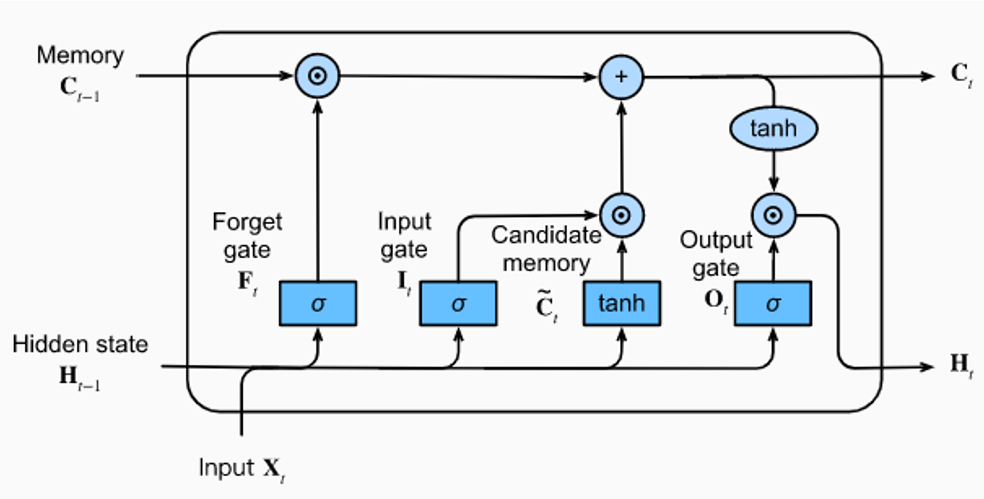
LSTM Architecture

Using the LSTM image above.

We have:

• $x_t$: our input at the current iteration
• $H_t-1$: our hidden state from the previous iteration
• $C_t-1$: our cell state from the previous iteration
• $\lambda = [H_t-1, x_t]$: the concatenation of the input and the previous hidden state
• $w_f$: Weights for the Forget Gate Linear Layer
• $b_f$: Bias for the Forget Gate Linear Layer
• $w_i$: Weights for the Input Gate Linear Layer
• $b_i$: Bias for the Input Gate Linear Layer
• $\tilde{C}_t$: The candidate cell state from the cell gate
• $\sigma$: The sigmoid function

1. The Forget Gate

• The input $x_t$ and the previous hidden state $H_t-1$ are concatenated into a single tensor, this is passed to the “Forget Gate” and will be represented as $\lambda$

• The “Forget Gate” is a Linear Layer that passes its product through a Sigmoid Function, the units will be converted to continuous values between $0-1$

• The product of the “Forget Gate” will then be multiplied by the cell state $C_t-1$, mutating a new cell state

• The multiplication acts as a way for the Model to “forget” a previous context if the output of the “Forget Gate” is a 0

• This is assumed that the LSTM Model will learn to “forget”, if the input signifies the end of a certain context e.g. an $xxbos$ token or a full stop or period.

• The formula for the product of the “Forget Gate”:

$f_t = \sigma(w_f * \lambda + b_f)$

2. The Input Gate and Cell Gate

• The Input Gate and Cell Gate act togther to update the new cell state $C_t$

• These gates decide whether to add a new piece of information to the long term memory

• The Input Gate takes the concatenated tensor and passes it through it’s linear layer to a Sigmoid Function

• The Cell Gate takes the same concatenated tensor and passes it through its Linear Layer through a TanH function

• The output of both gates are multiplied and then adds the cell state $C_t-1$

• The Input Gate essentially determines which units to update and the Cell Gate acts as determining the values for the update

• Input Gate:

$i_t = \sigma(w_i * \lambda + b_i)$

• Cell Gate:

$\tilde{C}_t = tanh(w_c * \lambda + b_c)$

3. The Output Gate

• The Output Gate is the final output of the LSTM Architecture

• The cell state $C_t-1$ is passed throught a TanH Activation Function

• The concatenated tensor is passed through the Output Gate Linear Layer and then through a Sigmoid Activation Function

• The product of the Sigmoid Function and the TanH function are multiplied leading to the new Hidden State $H_t$

• The cell state passes through without modification at this stage, leading to $C_t$

• The outputs $H_t$ and $C_t$ can be used in the next stacked LSTM Architecture

We can view the full formula for the new cell state:

$C_t = f_t * C_t-1 + i_t * \tilde{C}_t$

LSTMs pros

LSTMs improve on the Exploding/Vanishing Gradient problem over RNNs.

Since LSTMs use the cell state, the cell state is updated in an additive manner, the gradients backpropagating through the network are less prone to exploding/vanishing. Therefore, the magnitude of the gradients backpropagating through networks are not subject to as great of a variance as BPTT in RNNs.

LSTMs cons

• Like RNNs, LSTMs suffer from the lack of ability to parallelize the work, meaning slower and more computationally intensive training. LSTM requires contextual sequences to be trained in strict sequential order.

• The large number of parameters can also lead to overfitting

AWD-LSTM

ASGD Weight-Dropped Long Short Term Memory, is an optimized LSTM.

Compared to a vanilla LSTM, it uses Weight Dropping and ASGD (Averaged Stochastic Gradient Descent) to improve on overfitting.

Dropout

Dropout is a regularization technique that will randomly drop some activations in a Neural Net to zero. The theory behind Dropout is that the Neural Nets that are randomly dropped will force the Neural Net to form new connections, limiting the likelihood of the Neural Net to rely on specific neurons which could lead to overfitting.

It works by each neuron having a probability $p$ being dropped at the training stage.

Dropout is applied on every forward pass the Neural Network in training.

Bernoulli Distribution

Dropout is based on a straight forward Bernoulli Distrbution

Two possible outcomes:

• Success
• Failure

Probability of success: $q$

Probability of failure: $1 - q$

A simple example, flip a coin:

• success (heads) is $q = 0.5$

• failure (tails) is $1 - q = 0.5$

In terms of Dropout, the Bernoulli Distrbution is used to generate the binary mask.

• $p$ is the probability of dropping
• $q$ is the probability the neuron will be kept active

$q = 1 - p$

Binary Mask to deactivate neurons

• Using $p$, a Binary Mask is to generated so that certain neurons can be deactivated

• Using the code below as an example:

x = torch.tensor([0.1, 0.2, 5, 2, 3, 0.4])
p = 0.5
mask = x.new(*x.shape).bernoulli_(1-p)
mask

>> tensor([0., 1., 1., 0., 0., 0.])

• $p$ is set to 50% for deactivation of the neurons
• A Binary Mask is generated for a tensor of the same shape as the NN layer
• When the mask is applied, 50% of the neurons are deactivated, set to 0, each index of the mask represents which neurons to switch off

Scaling Outputs

With Dropout, the output needs to be scaled, since less neurons are active, the output will lower than it should be.

In order to scale the output to make up for less neurons being active, we need to apply the inverse of$p$ ($1-p$) to scale the output as if all the neurons were active.

Using the code example:

x * mask.div_(1-p)
>> tensor([0.000, 0.4000, 10.000, 0.0000, 0.0000, 0.0000])

Dividing the mask by $1-p$ will scale the outputs when applied to x, making up for the missing activations.

Activation Regularization and Temporal Activation Regularization

Activation Regularization (AR) and Temporal Activation Regularization (TAR) are regularization techniques that help prevent further overfitting and the exploding/vanishing gradient problem.

Similiarly to weight decay, AR and TAR apply penalizations to prevent overfitting but they are applied to the final activations themselves.

AR uses the L2 norm (squared magnitude) to apply a penality to the activations and then multiplies the product by a hyperparameter $alpha$

loss += alpha * activations.pow(2).mean()

• This prevents the activations from using very large values, preventing overfitting and exploding gradients

TAR, is similar to AR but is applied to sequential activations. Since LSTMs and RNNs are used to train sequential data, TAR applies a penalty to a sequence of activations to ensure the penalties are balanced over a sequence. This uses the beta hyperparameter.

loss += beta * (activations[:, 1:] - activations[:,:-1]).pow(2).mean()

It’s important to note, AR is applied to all neurons and TAR is only applied to the non-dropped neurons.

Transfomers

Transfomers have been arguably the most important and revolutionary Neural Network Architecture in recent times.

Transfomers are the basis for all the well known LLMs, GPT, BERT etc…

Transformers have a different mechanism from RNNs, where they don’t have any recurrent mechanisms, instead they used something known as self attention.

The basic transformer consists of an encoder and a decoder.

The encoder is responsible for generating outputs that represent a certain inputs relation (attention) to other tokens in an input. This might be a single word or subword in its positional relationship to the subwords around it.

TODO: Add a basic diagram of a table of words and its attention to the otehr words

The decoder is responsible for generating an output that can be used to calculate the predicted next token, based on the previously predicted token and the output of the encoder.

TODO: Add a basic diagram of a table of words, and the next likely word.

Below, I will step through in detail the model of a Transformer.

Encoder-Decoder

The Encoder-Decoder is a Transformer that utilizes both the encoder stack and decoder stack.

This type of transformer is especially effective when performing translations from one language to another.

Encoder

Input Embeddings

• The encoder begins with a text input that is preprocessed into tokens

• The purpose of generating Input Embeddings, is to be able to create continous variables that can be used when calculating the attention scores. This allows capturing the relationship of words to each other in a certain context.

• Each token has a word embedding generated for the token.

• A word embedding is a vector of random numbers (for GPT 512 numbers) mapped to the id in the vocab of the tokens

• Each word embedding is called an “Input Embedding”

• In the diagram below, we can see the final Input Embeddings of the words “How, are, you”.

• In the vocabulary, the tokens would be mapped to the Input Embedding, for example:

  • {"How": x1, "are": x2, "you": x3}
  • {x1, x2, x3} are the Input Embeddings, they are randomly generated numbers representing each word

class TokenEmbedding(nn.Module):
    def __init__(self, vocab_size, d_model):
        super(TokenEmbedding, self).__init__()
        self.embedding = nn.Embedding(vocab_size, d_model)

    def forward(self, x):
        return self.embedding(x)

Positonal Encoding

• A Positional Encoding is generated for each Input Embedding
  • A Positional Encoding is a vector of size n tokens.
  • The encoding is a vector of attendance of tokens to the other tokens
  • This uses sine and cosine to calculate the positions of each token in relation of each other
  • The will give us the basis for the attention mechanism, which is a models way of understanding, which words are most likely closer to each other
  • sine is applied to tokens in the even position and cosine is applied to tokens in the odd position
  • The Positional Encoding and original Input Embedding are added together to create the input into the next stage
  • This new output essentially has the Input Embedding with its positional information

This is the formula for calculating the Positonal Encodings:

• $PE(pos, 2i) = \sin\left(\frac{pos}{10000^{\frac{2i}{d_{model}}}}\right)$

• $PE(pos, 2i+1) = \cos\left(\frac{pos}{10000^{\frac{2i}{d_{model}}}}\right)$

• $pos$ = is the position of the token in the sequence

• $i$ = dimension index in the embedding vector

• $dmodel$ = total embedding size (e.g. 512 for GPT)

• $10000^{\frac{2i}{d_{model}}}$ = scaling factor to control frequency

class PositionalEncoding(nn.Module):
    def __init__(self, d_model, max_len=512):
        super(PositionalEncoding, self).__init__()

        pe = torch.zeros(max_len, d_model)

        for pos in range(max_len):
            for i in range(0, d_model, 2):
                pe[pos, i] = math.sin(pos / (10000 ** ((2 * i)/d_model)))
                pe[pos, i + 1] = math.cos(pos / (10000 ** ((2 * (i +1) / d_model))))

        # Add a batch dimension,when batched, it allows the Positional Encoding to be applied to `x` number of embeddings
        # according to the number in the batch dimension.
        pe = pe.unsqueeze(0)

        # positional encoding is saved as a buffer. It won't be used by an optimizer since its not a learnable parameter.
        # also ensure its moved to the correct device - CPU or GPU
        self.register_buffer('pe', pe)

    def forward(self, x):
        # The part where input embedding is added to the positional encoding for the corresponding input embedding.
        # self.pe[:, :x.size(1)] - slices the positional encoding tensor to match the length of input tensor x
        # x.size(1) gives the sequence length of the input tensor x.
        return x + self.pe[:, :x.size(1)]

Multi Head Attenion Mechanism

• The input (Embedding with positional context) is passed to the Multi Head Attention Mechanism

• The MHA takes the input and creates x3 copies:

  • Q (queue): The current token to be processed. This token is used to score against all the other tokens using K.
  • K (key): The tokens that will be used in comparison to the Q token.
  • V (value): The original value of the token.

Each Q, K, V are calculated by multiplying the input embedding with each respective weights:

• $Q = Xi * Wq$
• $K = Xi * Wk$
• $V = Xi * Wv$

The output of the MHA is:

• For each $Q$, calculate its attendence for each $K$

• $attention score = QK^t$

• t means transpose, in order to get the output vector of a certain size n, we need to transpose K

• The attention_score is a vector of probabilities against the other tokens, this gives us an attention score on the probabilitity of which words come next

This is a crude demonstration of the attention score:

Token: <In>
                  the  house was  ....
Attention Score: [0.2, 0.6,  0.2, ....]

• In order to increase the performance of the results, MHA uses a number of $heads$. This essentially creates $N$ number of vectors by splitting the vector size among the heads.

• This in theory and practice, allows the split to concentrate on different relationships in the input. The output of all the split heads are recombined to form the attention score.

After the attention scores are calculated, we need to scale the outputs:

• $\frac{QK^T}{\sqrt{d_k}}$

• Square root of $d_k$ is the square root of the embedding size

• Then the output is put through a softmax function that smooths out the outputs to be between ${0..1}$

• Then the attention score is multiplied by V, giving the final attention output

• Its important to note:

  • The attention score is a vector with the attention to each word
  • $V$ is the word embedding
  • The output is a word embedding with the contextual information of the attention_score

Below is an example of attention scores from the MHA for each token in relation to other tokens:

The final output of the MHA is a multiplication of the vector of attendance (like above) with the vlaue vectors (which are dervied from the word embeddings). This creates an output vector that has the word embedding with the word attendence combined (containing contextual information).

class MHA(nn.Module):
    def __init__(self, heads, d_model):
        super(MHA, self).__init__()
        # d_k is the dimensionality of each of the attention heads, e.g. 512 d_model // 8 heads = 64 dimeinsional subspace for each attention head
        self.d_k = d_model // heads

        # Number of attention heads for K,Q,V
        self.heads = heads

        self.W_q = nn.Linear(d_model, d_model)
        self.W_k = nn.Linear(d_model, d_model)
        self.W_v = nn.Linear(d_model, d_model)

        # fully connected layer will be used to gather and combine the outputs of the self attention calculation.
        self.fc = nn.Linear(d_model, d_model)
        self.attention = ScaledDotProduct(self.d_k)

    def forward(self, Q, K, V, mask=None):
        # TODO: Is this getting it from the batch size index?
        batch_size = Q.size(0)

        # View creates multiple copies of the each head according to heads
        # self.W_x calls forward on X and the Linear Layer
        # view(...) Splits into multiple heads, according to self.heads
        # transpose(1,2), swaps positions 1 and 2.
        #    prev: [batch_size, seq_len, heads, d_k]
        #    after:  [batch_size, heads, seq_len, d_k]
        # This allows parallel computation for each head
        Q = self.W_q(Q).view(batch_size, -1, self.heads, self.d_k).transpose(1, 2)
        K = self.W_k(K).view(batch_size, -1, self.heads, self.d_k).transpose(1, 2)
        V = self.W_v(V).view(batch_size, -1, self.heads, self.d_k).transpose(1, 2)

        scores, attn = self.attention(Q, K, V, mask)

        # Combine all the heads back into one vector per token
        scores = scores.transpose(1, 2).contiguous().view(batch_size, -1, self.heads * self.d_k)
        output = self.fc(scores)
        return output

Add + Norm

The output of the MHA is normalized via the Add + Norm layer.

The attention_score is added to the original Embedding with positional context. The pre-MHA Word Embedding is added together with the output of the MHA and passed to the LayerNorm function for normalization:

• $LayerNorm(Word Embedding + MHA Output)$

The output is put through a LayerNorm function.

This stabilizes the function around a mean and variance of the mean being 0 and the variance being 1.

$LayerNorm = x - u / o * y + B$

$x$: input

$u$: mean across all dimensions

$o$: standard deviation

$y$: scale

$B$: bias

Feed Forward

This is put through a Feed Forward Network, this expands the original embedding size and performs a ReLu on the input.

GPT, expansion of 512 dimensions to 2048

• $Xw1 + b1$
• $FFN(X) = ReLu(Xw1 +b1) * W2 + b2$

# Feedforward Layer
class FeedForward(nn.Module):
    # d_ff is the feed foward layer's hidden layer size
    def __init__(self, d_model, d_ff, dropout=0.1):
        super(FeedForward, self).__init__()
        self.fc1 = nn.Linear(d_model, d_ff)
        self.fc2 = nn.Linear(d_ff, d_model)
        self.dropout = nn.Dropout(dropout)
        self.relu = nn.ReLU()

    def forward(self, x):
        x = self.dropout(self.relu(self.fc1(x)))
        x = self.fc2(x)
        return x

Second Add + Norm

The second Add + Norm repeats like the previous Add + Norm but uses:

• The Feed Forward output + the output of the first Add + Norm (before sending it to the Feed Forward )

This is the final output of the encoder which gives an output of an Embedding for each token that has contextual information about the attendence scores with other tokens in the same context

$LayerNorm()$

Encoder Summarized

class EncoderLayer(nn.Module):
    def __init__(self, d_model, heads, d_ff, dropout=0.1):
        super(EncoderLayer, self).__init__()
        self.attention = MHA(heads, d_model)
        self.norm1 = nn.LayerNorm(d_model)
        self.ff = FeedForward(d_model, d_ff, dropout)
        self.norm2 = nn.LayerNorm(d_model)
        self.dropout = nn.Dropout(dropout)

    def forward(self, x, mask=None):
        # Multi-head attention with residual connection and layer normalization
        attn_output = self.attention(x, x, x, mask)
        x = self.norm1(x + self.dropout(attn_output))

        # Feedforward network with residual connection and layer normalization
        ff_output = self.ff(x)
        x = self.norm2(x + self.dropout(ff_output))
        return x

class Encoder(nn.Module):
    def __init__(self, vocab_size, d_model, N, heads, d_ff, dropout=0.1):
        super(Encoder, self).__init__()
        self.embedding = TokenEmbedding(vocab_size, d_model)
        self.positional_encoding = PositionalEncoding(d_model)

        self.layers = nn.ModuleList([EncoderLayer(d_model, heads, d_ff, dropout) for _ in range(N)])
        self.dropout = nn.Dropout(dropout)

    def forward(self, x, mask=None):
        x = self.embedding(x)
        x = self.positional_encoding(x)

        for layer in self.layers:
            x = layer(x, mask)

        return x

Decoder

The decoder is the second stage of a transfomer. Its the stage that generates the probabilities of the next token given a token input.

The Decoder takes x2 inputs:

• The output generated by the encoder (the token embedding with attenion context)
• For inference:
  • The previously generated token, if its the beginning of a generation, then a special character indicating start of stream
• For training:
  • The target variable (the next word)

Like the encoder, the previously generated token has their embedding generated and then their Positional Encoding generated.

The Positonal Encoding and token embedding are added together

Masked Multi Head Attention

The same approach as Multi Head Attetion, generating the K,Q,V by copying the input and multiplying by weights.

This approach differs because the masked element, makes future tokens in the attention vector voided out. This essentially means the model cannot see the next token, it can only attend to its previous tokens.

This is achieved by setting the future tokens in the context to 0

The output of the attention score is outputted to the Add and Norm stage.

Add + Norm

Add norm takes the maked MHA output and adds it with the original input with postional embedding context

This performs LayerNorm to stablilize around a mean and variance.

Second MHA

There is a second multi head attention that is used with the Encoder output as the Q, and the normalized output of the masked MHA as the K and V.

Add + Norm

• Output of the first Add + Norm and MHA is used in Add + Norm
• The does LayerNorm and stabilizes around mean and norm stage

Feed Forward

• Through the same Feed Forward

Add + Norm

• Output of Feed Forward and the output of the previous Add + Norm

Linear + Softmax

• Converts the output of a 512d token embedding to a list of probabilities of the next token
• Uses softmax(final decoder output + W_vocab + b_vocab)

Output Probabilities

• The output is a list of the predictions of the next word e.g.

{ “Le”: 0.92, “Un”: 0.05, “Il”: 0.03}

Decoder Only

TODO:

BPE (Byte Pair Encoding)

BPE is a common tokenizing strategy used in LLMs such as GPT and BERT.

BPE is a greedy algorithm that finds the most common subtokens to build a vocabulary.

How BPE Works

1. Initialize the symbols

Each word is initially split into individual characters and end-of-word markers </w.

It then counts all adjacent symbol pairs.

lower</w>

l o
o w
w e
e r
r </w>

2. Count Symbol Pair Frequencies

It then finds the count of the token pairs.

It then merges the most frequent pairs.

e.g.

pair_freq = {
    ("l", "o"): 5,
    ("o", "w"): 3,
    ...
}

3. Merge the most frequent pair

If l o is frequent, it becomes lo. This continues until the max vocabulary size is achieved.

4. Update the Vocabulary

vocab = {
    "lo", ...
}

5. Repeat until max size reached

This restarts the steps until the max vocabulary size is reached or there is nothing left to merge.

The final vocabulary might look like:

low
er
est
ne
new

Why is BPE used?

• No OOV (out of vocabulary) problem, all text is representable if the vocabulary corpus was sufficiently large enough
• Simple and language agnostic

Example use of BPE

The transformer tokenizer has a BPE class:

• The BpeTrainer is the class that executes counting the symbol pairs and applies the merges.
• The BPE class is a wrapper that stores the vocabulary, the special token mapping and the rules.

from tokenizers import Tokenizer
from tokenizers.models import BPE
from tokenizers.trainers import BpeTrainer
from tokenizers import normalizers
from tokenizers.pre_tokenizers import Whitespace
from tokenizers.normalizers import NFD, Lowercase, StripAccents

tokenizer = Tokenizer(BPE(unk_token="[UNK]"))
tokenizer.normalizer = normalizers.Sequence([NFD(), Lowercase(), StripAccents()])
tokenizer.pre_tokenizer = Whitespace()

trainer = BpeTrainer(special_tokens=["[UNK]", "[CLS]", "[SEP]", "[PAD]", "[MASK]"], vocab_size=5000)

GPT2

This section will briefly cover GPT2 which is a well known decoder only transformer.

GELU

GPT2 uses GELU (Gaussian Error Linear Unit). GELU is an activation function that applies a smooth and probablistic gating to inputs. It is different to ReLU where GELU is a less harsh gating function. Negative numbers and small positive numbers will be smoothed out gradually instead of the sharp cutoff of ReLU, leading to the model able to retain small signal information.

Weight Tying

GPT2 uses Weight Tying, which means the input token embeddings share the same weights as the output layer. This has advantages of reducing the number of parameters in the model and introduces consistency in how the tokens are represented and how they are predicted.

Learnable Positions

GPT2 doesn’t use the sin/cosine positional encoding formula like in the classic encoder-decoder transformer.

GPT2 uses a tensor of embeddings for each index relative to the token embeddings. During backpropagation, the postional encodings are updated based on the predictions, meaning the positional embeddings are adjusted due to their predictions indicating their likely positions.

DeepSeek

Uses:

• Grouped Query Attention (GQA)/Multi Latent Attention

Grouped Query Attention/Multi Latent Attention

• Builds on MHA and Multi-Query Attention

• MHA creates a K,Q,V for every head

  • High expressiveness but high memory and compute cost

• MQA uses the same K,V across all heads but keeps Q independent on each head

  • Faster and less compute power but may degrade quality

GQA is a hybrid approach of MHA and MQA

It’s more performant than MHA but more efficient than MQA.

1. Divide query heads into G groups (8 query heads -> 2 groups of 4 heads)

2. Each group shares a single K and V

3. Independent Q per head inside the group

E.g.

Group 1: Heads 1-4 share K1, V1 Group 2: Heads 5-8 share K2, V2

• Each head within each group has its own Q.

The goal is to reduce memory and compute cost

Advantages

• Faster then MHA

• Higher quality than MQA

• Also used in LLaMA-2 (70B)

Sliding Window Attention TODO: I’m not sure it uses this

A technique to further reduce memory cost when it comes to masking.

It limits the attentendence of tokens to a window of size W.

The means the sliding window attention maybe be [i-w], e.g. W=4 and token position index is 5 = [2, 3, 4, 5].

This has an improvement from quadratic to linear time O(n * w) and is more memory efficient.

But it may loose global information as its focus is on local information.

• its used in Mistral 7B and DeepSeek-Long

LayerNorm before MHA

LayerNorm in DeepSeek is applied before passing the MLA

RMSNorm (Root Mean Square Norm)

A simplified version of LayerNorm:

• Removes the mean centering step
• Keeps the rescaling step
• Is fast and more memory-efficient

In the equation, it just removes the mean variable and learned bias.

$\text{RMSNorm}(x) = \frac{x}{\text{RMS}(x) + \epsilon} \cdot \gamma$

RoPE - Rotary Position Encodings

TODO: Basically calculating the positions of tokens inside the attention mechanism.

• Rotates the querys/keys in the multi head attention?

Flow:

1. Generate K,Q,V

2. Apply RoPE to Q and K, this rotates each positions vector

3. $\theta_{p, i}$ is the rotation angle, calculated from the position token and the head dimension, similar to the original positional embedding in encoder-decoders.

4. RoPE is applied for each $qp$ and $kp$, converting into pairs $(q2i, q2i + 1)$ and $(k2i, k2i+1)$

• Rotate the Query Pair:

• Rotate the Key Pair:

5. Concatenate all Rotated Pairs

• All pairs $(\hat{q}_2i, \hat{q}_2i + 1)$ are concatenated to form $\hat{q}_p$
• All pairs $(\hat{k}_2i, \hat{k}_2i + 1)$ are concatenated to form $\hat{k}_p$

6. Compute the attention scores using the dot product of each concatenated tensor $\hat{q}_p$ and $\hat{k}_p$

6. Apply softmax to the score, then multiply by $V$

7. Output to the next layer

Because Q and K are different tokens, when we are attending to it with attention, we can also convert their absolute distance to relative distance and bake it straight into the attention score.

Advantages

• Positions are baked into the attention output creating sensitivity to relative distances
• No extra memory or parameters required
  • RoPE is calculated in-place with the positional embeddings in the attention output
  • No additional positional embeddings required
  • No weights for positional embedding required therefore less computation on backpasses

SwiGLU - Swish-Gated Linear Unit

SwiGLU is a variation of Gated Linear Unity.

Essentially splits the input into two parts:

• A gated part that uses the Swish activation function and the other non-gated.

They are multiplied together to get the otuput.

Flash Attention

A GPU-optimization for attention calculation using memory efficient blocks and streaming softmax.

It enables faster training and longer sequence lengths.

Mixture of Experts

Instead of a dense MLP layer, multiple MLP layers are used but only a few are activated when going through a pass. Each expert has its own weigts.

Each Expert may begin to specialise, e.g. expert 1 is common language, expert 5 rare or technichal wrods.

A router ( a tiny neural net of linear layer and softmax) will route each token to a certain expert.

TODO:

• Router (Linear Layer), outputs logits for each index position for each expert

• The logits are element-wise added to Gaussian noise, this is only performed in training to improve load-balancing to experts, this is performed before softmax

• The logits are passed to a softmax function, this gives us the probabilities for each expert

• Top K experts are chosen for routing based on the softmax output, K is a hyperparameter

• The inputs are routed to the activated expert

• Each expert outputs a tensor

• The tensors are combined using a weighted sum, where p1 and p2 are renormalized routing weights: final_out = p1 * Expert(1) + p2 * Expert(2)

Advantages

• MoE only activates a few experts, good for big models, faster inference

• Allows capturing knowledge without directly increasing the parameters

• Prevents overfitting sicne experts dont see all the same data

THOUGHTS TODO:

• Is there a trade off in learning and scalability?
  • e.g. Moving the positional encoding to the GQA to save time and space.

Architecture

Architecture Overview

• Type: Decoder-only autoregressive transformer

Tokenizer

Byte-Pair Encoding with a large vocabulary of (~100k to 200k tokens).

It includes special tokens for padding, BOS/EOS and task specific tokens for instruction tuning.

Transformer Layers

• Depth: 60-100 layers depending on model size (e.g. 80 layers for 70B parameter)

• Pre-Normalization: RMSNorm applied before attetion and FFN layers for stability

Flow

TODO: Upload diagram from draw.io

hidden_state <---
|               |
V               |
                |
RMSNorm         |
|               |
V               |
                |
MLA             |
|               |
V               |
                |
residual_conn <->
                |
|               |
V               |
                |
RMSNorm         |
                |
|               |
V               |
                |
FFN/MLP         |
                |
|               |
V               |
                |
residual_conn <--

|
V

output

Attention Mechanism

Multi-Head-Attention: Using Multi Latent Attention/Grouped Query Attention, 32-64 heads per layer.

Feed-Forward Network (FFN)

• SwiGLU Activation
• MoE Integration

Did you find this page helpful? Consider sharing it 🙌