Neural Networks 101: Part 2 - Neural Network Maths

This post will go through the maths and the implementation details on how a Neural Network learns.

This is still very much an overview and foundation of Neural Networks, this post won’t go into details about certain Neural Networks.

This post assumes you have read Neural Networks 101: Part 1, go read that if you haven’t already.

How does a Neural Network learn?

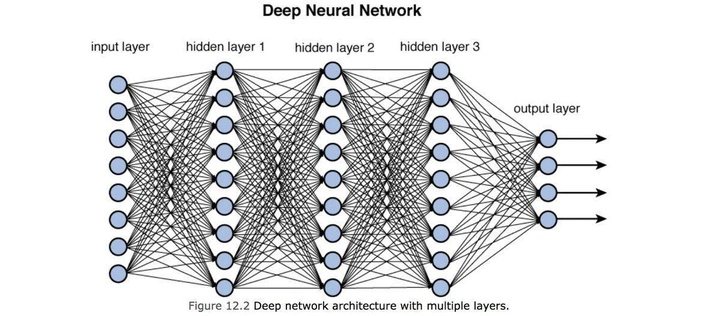
In Part 1, we went through the basic model of a Neural Network as seen in the diagram below.

We are going to create a new diagram that helps in our understanding of the learning process.

The above diagram is still applicable for understanding the model of a Neural Network but the diagram below will demonstrate the process of learning.

The “learning” diagram has the following steps:

INIT: initailize the PARAMETERS
PREDICT: For each input, predict whether the input matches a LABEL
LOSS: Based on the predictions, calculate the accuracy of the prediction
GRADIENT: Calculate the gradient, a variable that determines how much to adjust the PARAMETERS to affect the LOSS
STEP: Adjust the PARAMETERS based on the calculated gradient
Repeat the process again, going back to PREDICT while using the newly adjusted PARAMETERS
STOP: Continue this iterative process until the level of loss is acceptable

We can see that this learning mechanism, calculates the required changes to adjust PARAMETERS in order to bring the LOSS to an acceptable level.

In the next section we’ll go into detail on each componenet.

Randomized Parameters and the Universal approximation theorem

The first part of our diagram is INIT, at this stage we randomly initailize our PARAMETER values.

The idea of randomizing the PARAMETERS is partly inspired by the Universal approximation theorem.

This theorem states that given a Neural Network with sufficient neurons, it can approximate any continuous function.

Therefore, the PARAMETERS can be initialized to almost any state since the process of iteratively adjusting the weights according to the calculated gradients enables the Neural Network to adapt and refine its accuracy, effectively learning the function it needs to model.

SGD (Stochastic Gradient Descent)

After we’ve calculated our PREDICTIONS and determined the LOSS. We need to update our PARAMETERS to improve the accuracy of our PREDICTIONS.

Stochastic Gradient Descent is an optimization method used in Neural Networks to refine the PARAMETERS. SGD calculates the GRADIENT (a derivative) of the LOSS.

This is essentially a measure of the rate of change between the PREDICTIONS and the LABELS.

The calculated GRADIENT provides a direction and magnitude indicating how the PARAMETERS should be adjusted to minimize the LOSS. The adjustment is made by moving the PARAMETERS in the opposite direction of the gradient, scaled by a learning rate (the step size).

By applying these steps iteratively the model gradually improves its performance.

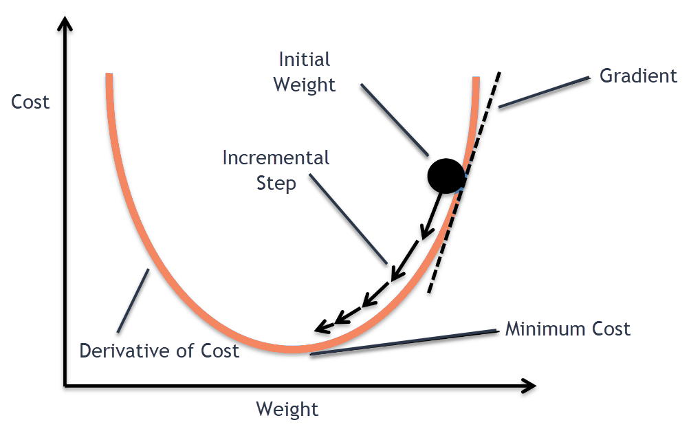
Derivatives

As a quick refresher on the maths in SGD.

A derivative is a value that represents a rate of change at a certain point towards the critical point.

Using the limit notation of a derivative function, we can find the derivative.

f'(x) = \lim_{h \to 0} \frac{f(x+h) - f(x)}{h}

We can understand derivatives by using a simple example.

Let’s assume a company has a profit function:

P(x) = -2x^2 + 12x - 10

Let’s assume the profit function has a quadratic form that indicates, as revenue increases with each unit sold, theres a point where increased production leads to diminishing returns.

The objective is to find the number of units x, that maximizes profit.

Substitue x for (x + h) from derivative equation.

f(x + h) = -2(x + h)^2 + 12(x + h) - 10

Expand P(x + h)

f(x + h) = -2(x^2 + 2xh + h^2) + 12x + 12h - 10

f(x + h) = -2x^2 - 4xh - 2h^2 + 12x + 12h - 10

Calculate P(x + h) - P(x):

f(x + h) - f(x) = (-2x^2 - 4xh - 2h^2 + 12x + 12h - 10) - (-2x^2 + 12x - 10)

f(x + h) - f(x) = (-2x^2 - 4xh - 2h^2 + 12x + 12h - 10) + 2x^2 - 12x + 10

f(x + h) - f(x) = -4xh - 2h^2 + 12h

Divide by h and simplify:

f'(x) = \lim_{h \to 0} \frac{f(x+h) - f(x)}{h} = \frac{-4xh -2h^2 + 12h}{h}

f'(x) = \lim_{h \to 0} f(x+h) - f(x) = -4x -2h + 12

Apply the limit as h approaches 0:

f'(x) = \lim_{h \to 0}(-4x -2h + 12)

f'(x) = -4x + 12

We can see that given our Profit function, we have our derivative function:

P'(x) = -4x + 12

This function tells us the magnitude and rate of change towards the limit 0, as the production quantity x changes.

If we set $P'(x) = 0$ , we will be able to find the level that maximizes profit. This works because we are creating a linear equation where we are solving for x given 0, the critical point.

-4x + 12 = 0

-4x = 12

x = \frac{12}{4}

x = 3

We can see that the critical point is reached using the value $x = 3$ . In this example, this means that to maximize profit, the company only needs to produce 3 items, any more or less moves away from the critical point resulting in a loss or missed profit.

In the context of Neural Networks, let’s say that 3 is our target. By using other values such as $x = 12$ in our derivative function, the derivative value will essentially tell us the rate of change towards or away from the critical point 3.

We can use this derivate value (the GRADIENT) in SGD to step our PARAMETERS. This means we are adjusting x towards a value that will get us closer to 3.

Calculating the GRADIENTS from the LOSS is known as Back Propagation.

Step

Now that we’ve understood the maths behind Back Propagation. The SGD optimization process requires the use of the calculated GRADIENTS to update the initial PARAMETERS.

This where the STEP phase is applied. This phase subtracts the PARAMETERS by the calculated GRADIENTS but using a learning rate.

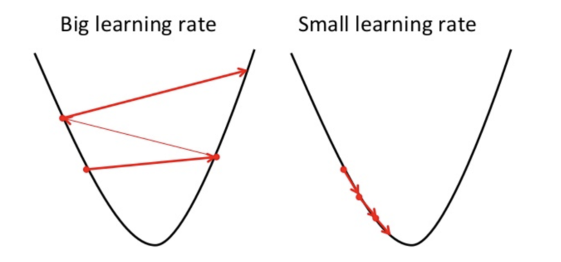
The learning rate is an important variable because too big of a learning rate, the PARAMETERS may vary widly in value but too low of a learning rate, the PARAMETERS won’t effectively be updated sufficiently.

The process of finding and using an appropriate learning rate is important and won’t be convered in this article.

Stop

This is the final phase. After several rounds of making predictions, calculating the loss, calculating the gradients and the stepping the parameters. We should reach a stage where the loss has been reduced to an acceptable level, the training of the Neural Network is stopped.

At this point, we no longer need to perfom training iterations (epochs). The Neural Network could now be used to make predictions on unseen input.

Summary

In this article, we have explained at a high level the process of how a Neural Network learns and the maths behind it.

We identified an optimization technique called Stochastic Gradient Descent.

Initialize a random set of PARAMETERS. We can use ranzomied values due to the Universal approximation theorem
Generate a PREDICTION based on the training input and the corresponding LABEL
Calculate the LOSS of the PREDICTION, essentially a value measuring the performance of the PREDICTION against the LABEL
Calculate the GRADIENT. This a derivative of the LOSS, telling us the magnitude and direction from the critical point (the correct LABEL)
Step the PARAMETERS. By using a learning rate as a scalar variable, we subtract the PARAMETERS by the GRADIENT. This should move our PARAMETERS in a direction that should reduce the LOSS, meaning future PREDICTIONS will become more accurate
Stop. Once we have seen the LOSS decrease to an acceptable level, we can stop training the Neural Network

In Part 3, I will go into detail of a Neural Network